Comparison of data dimensionality reduction methods!

Principle Component Analysis

One of the benefits of the tidymodels ecosystem is the flexibility and ease of trying different approaches for the same kind of task. With function recipe, you don’t have to perform every step, you only need to write them down.

library(tidymodels)

pca_rec <- recipe(~ ., data = cocktails_df) %>% 
  update_role(name, category, new_role = "id") %>% 
  step_normalize(all_predictors()) %>% 
  step_pca(all_predictors(), num_comp = 2)

pca_prep <- prep(pca_rec)

pca_prep

Here, let’s focus on the variable pca_rec, what we have done is:
- First, tell recipe() what’s going on with our model and what data we are using. - Second, we update the role of name and category columns by function update_role(), since these are variables we want to keep around as identifiers for rows. - Then we need to center and scale the numeric predictors. - Finally, we use step_pca for the actual principal component analysis. Note that actually, the PCA step is the second step. The prep estimate the required parameters from a training set that can be later applied to other datasets for us.

Once we have our recipe done, we can explore the results by using tidy(), which makes it possible to visualize what each components look like.

tidied_pca <- tidy(pca_prep, 2)

tidied_pca %>% filter(component %in% paste0("PC", 1:5)) %>% 
  mutate(component = fct_inorder(component)) %>% 
  ggplot(aes(value, terms, fill = terms)) + 
  geom_col(show.legend = FALSE) + 
  facet_wrap(~component, nrow = 1) + 
  labs(y = "")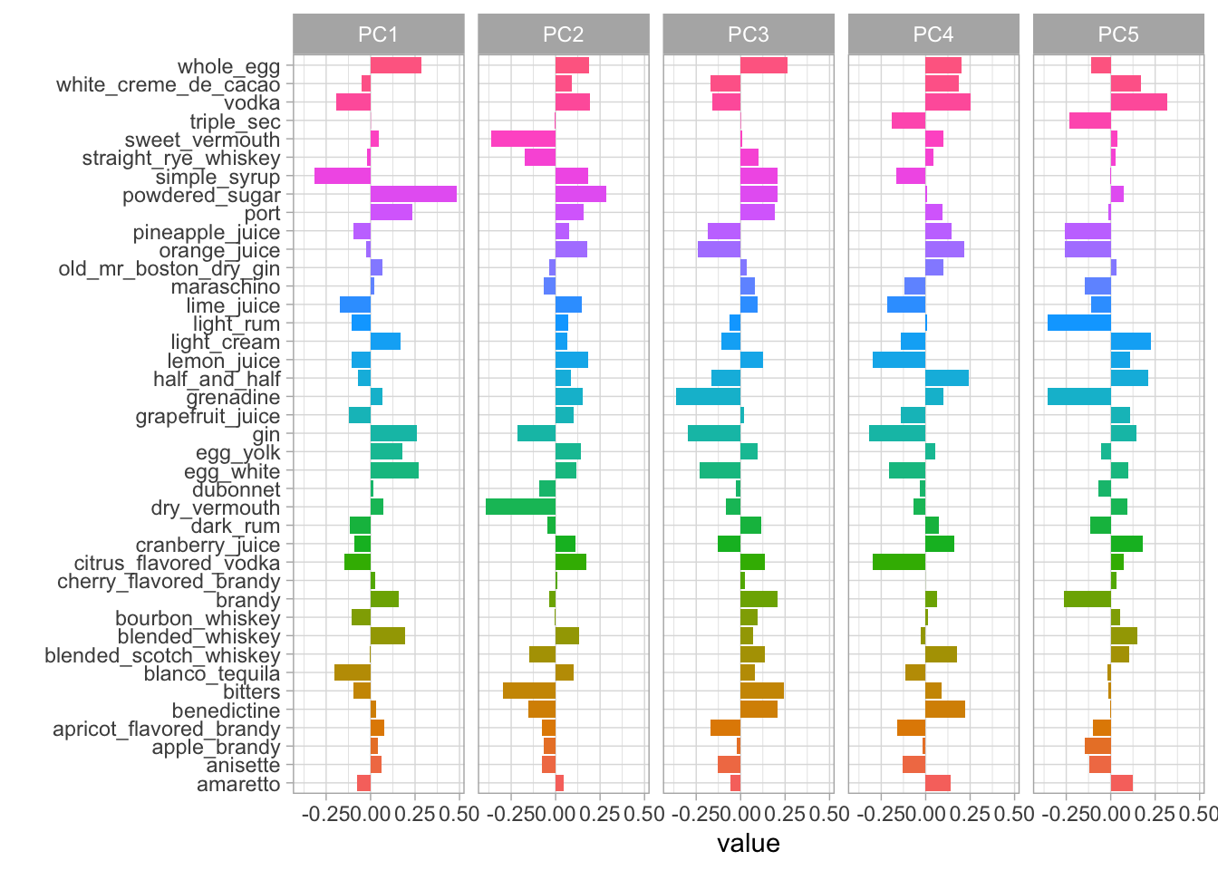

In the plot above, we can see how much every component contributes to each category. Clearly, the biggest difference in PC1 is powdered sugar vs. simple syrup. Let’s zoom in on the first four components, and understand which cocktail ingredients contribute in the positive and negative directions.

library(tidytext)

tidied_pca %>% 
  filter(component %in% paste0("PC", 1:4)) %>% 
  group_by(component) %>% 
  top_n(8, abs(value)) %>% 
  ungroup() %>% 
  mutate(terms = reorder_within(terms, abs(value), component)) %>% 
  ggplot(aes(abs(value), terms, fill = value > 0)) + 
  geom_col() + 
  scale_y_reordered() +
  facet_wrap(~component, scales = "free_y") + 
  labs(fill = "positive?")

So PC1 is about powdered sugar + egg + gin drinks vs. simple syrup + lime + tequila drinks. This is the component that explains the most variation in drinks. PC2 is mostly about vermouth, both sweet and dry.

bake(pca_prep, new_data = NULL) %>%
  ggplot(aes(PC1, PC2, label = name)) +
  geom_point(aes(color = category), alpha = 0.7, size = 2) +
  geom_text(check_overlap = TRUE) +
  labs(color = NULL)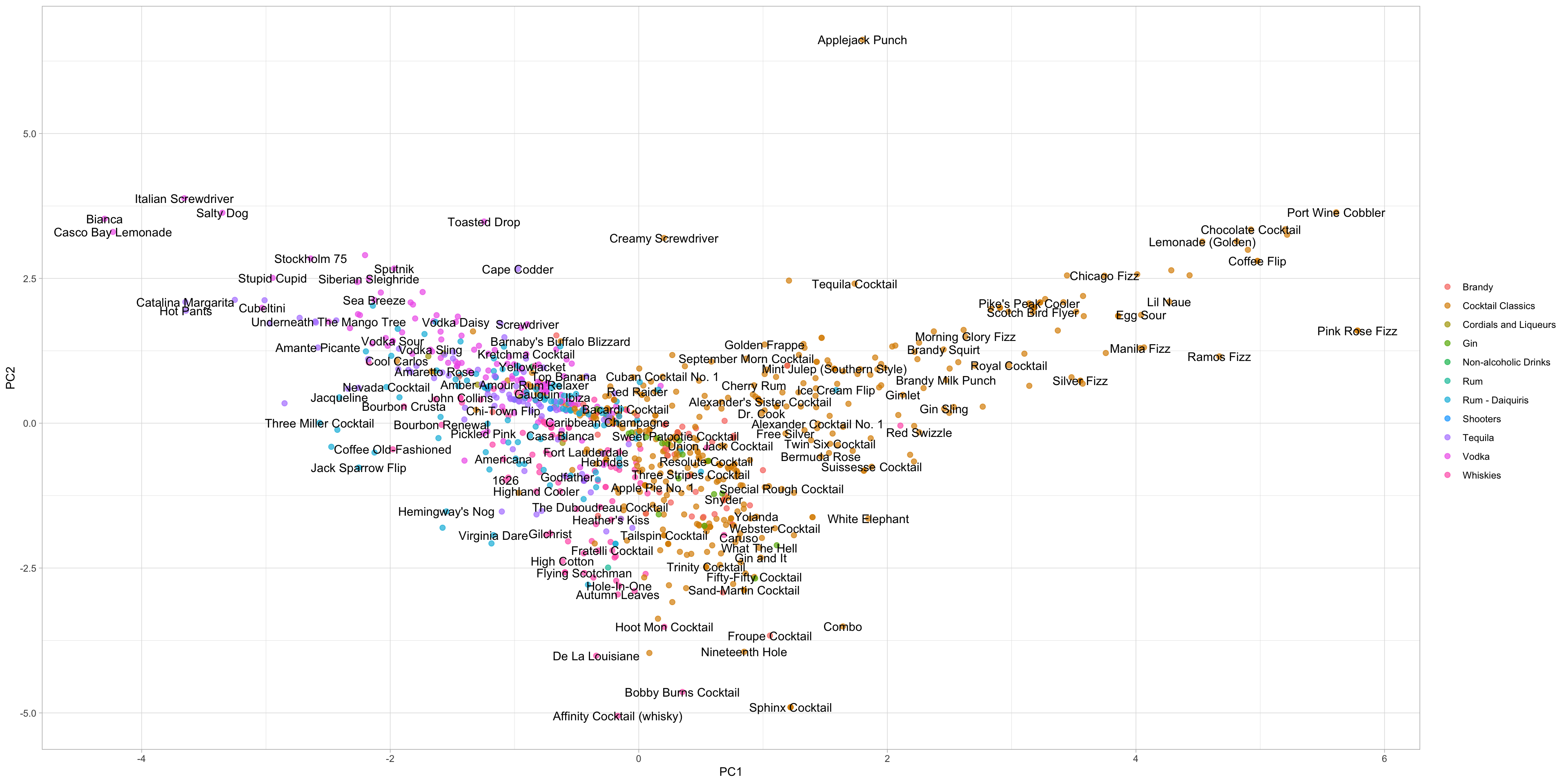

The plot above shows how the cocktails distributed in the plane of the first two components. The bake() return the computations accroding to the recipe. We can conclude: - Fizzy, egg, poweder sugar drinks are to the left. - Simple syrup, lime, tequila drinks are to the right. - Vermouth drinks are more to the top. Although many labels are mixed together, they may be distinguishable on other components.

Uniform manifold approximation and projection

Thanks to the benefits of the tidymodels ecosystem, we can switch out PCA for UMAP, simply by replace step_pca() by step_umap. Before that, don’t forget to import package embed, which provide recipe steps for ways to create embeddings including UMAP.

library(embed)

umap_rec <- recipe(~ ., data = cocktails_df) %>% 
  update_role(name, category, new_role = "id") %>% 
  step_normalize(all_predictors()) %>% 
  step_umap(all_predictors(), num_comp = 5)

umap_prep <- prep(umap_rec)

umap_prep

Similarly, we can see how the cocktails are distributed in the plane of the first two UMAP components.

bake(umap_prep, new_data = NULL) %>%
  ggplot(aes(umap_1, umap_2, label = name)) +
  geom_point(aes(color = category), alpha = 0.7, size = 2) +
  geom_text(check_overlap = TRUE) +
  labs(color = NULL)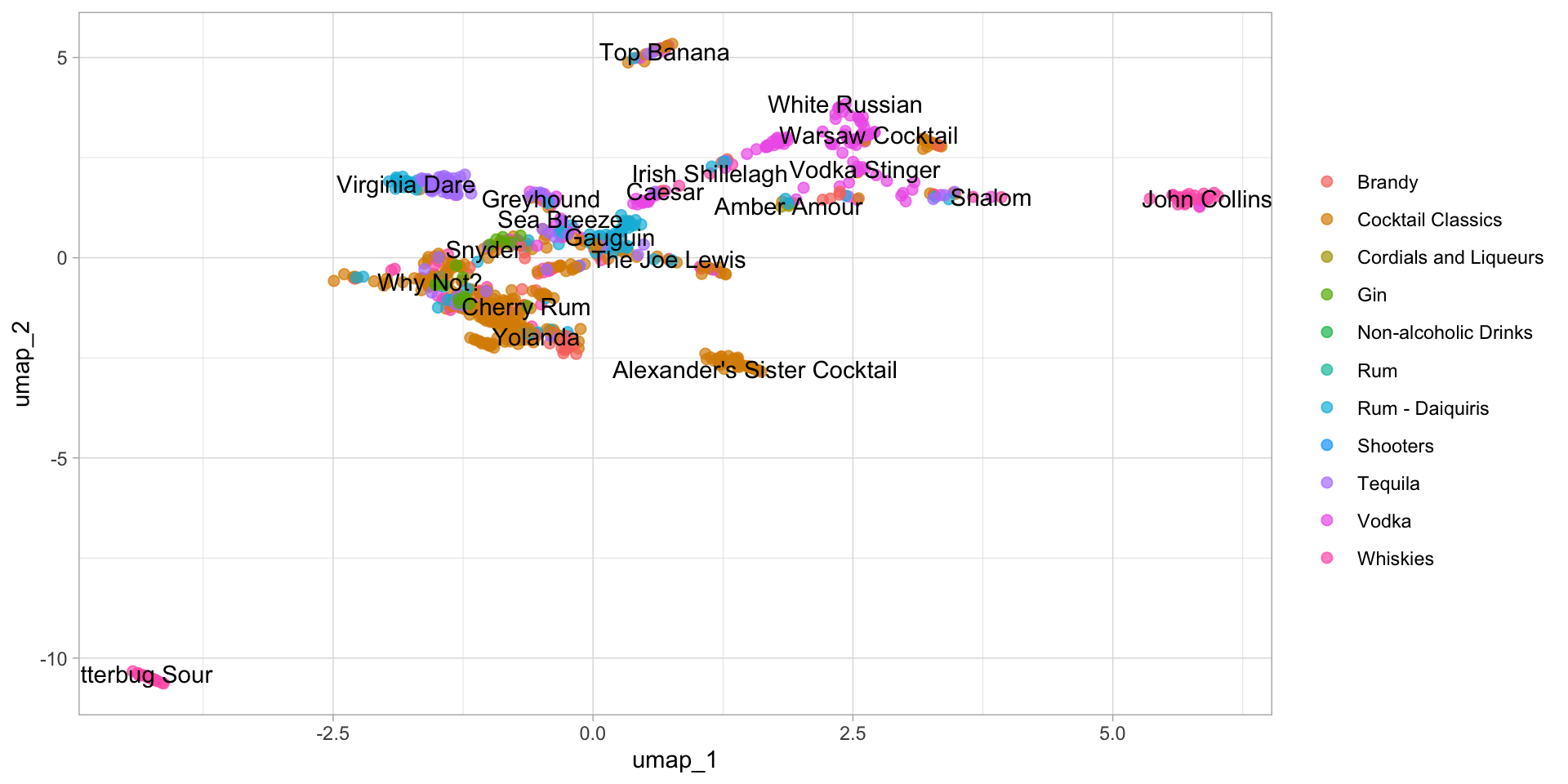

You can see that the distribution of the first two components of UMAP is totally different from PCA. Obviously, most of the categories didn’t mix together. That’s what I’m talking about. And I can tell, the performance of the classification algorithm trained on the first two components of UMAP will definitely better than of PCA. Let’s prove it on the kernel SVM (Support Vector Machine).

library(e1071)

svm_test <- function(num_compo, meth){
  if(meth == "PCA"){
    rec <- recipe(~ ., data = cocktails_df) %>% 
    update_role(name, category, new_role = "id") %>% 
    step_normalize(all_predictors()) %>% 
    step_pca(all_predictors(), num_comp = num_compo)
  }
  
  if(meth == "UMAP"){
    rec <- recipe(~ ., data = cocktails_df) %>% 
    update_role(name, category, new_role = "id") %>% 
    step_normalize(all_predictors()) %>% 
    step_umap(all_predictors(), num_comp = num_compo)
  }
  
  df <- bake(prep(rec), new_data = NULL)
  
  n <- nrow(df)
  ntrain <- round(n * 0.75)
  set.seed(123)
  
  tindex <- sample(n, ntrain)
  train_iris <- df[tindex, ]
  test_iris <- df[-tindex, ]

  svm1 <- svm(category~., data = train_iris, method = "C-classification", 
              kernal="radial", gamma = 0.1, cost = 10)
  
  prediction <- predict(svm1, test_iris)

  xtab <- table(test_iris$category, prediction)
  result <- data.frame(test_iris$category, prediction)
  accuracy <- sum(test_iris$category == prediction) / nrow(test_iris)
  return(accuracy)
}

Here is a function require two variables input, the number of component and demensionality reduction method, and output the accuracy of the classification. Let’s first verify the performance of the first two components.

cat("PCA: ",svm_test(2, "PCA"), ", UMAP: ",svm_test(2,"UMAP"))

## PCA:  0.6410256 , UMAP:  0.7051282

Obviously, the first two components of UMAP contains more classification information, at least make the SVM classify more accurate.

You think that’s the end of it? We know that, in real life, we should always consider the time cost, and that is the meaningful of the dimensionality reduction method. So let add the time cost into the comparision, start by finding out how many components PCA needs to achieve the same accuracy as UMAP.

result_pca <- 1:10 %>% map_dbl(svm_test, meth = "PCA") 
result_umap <- 1:10 %>% map_dbl(svm_test, meth = "UMAP") 
result <- data.frame(pca = result_pca,
                     umap = result_umap) %>% stack()

result$index <- c(1:10,1:10)

result  %>% 
  ggplot(aes(index, values, color = ind)) + 
  geom_line() + 
  labs(color = "method")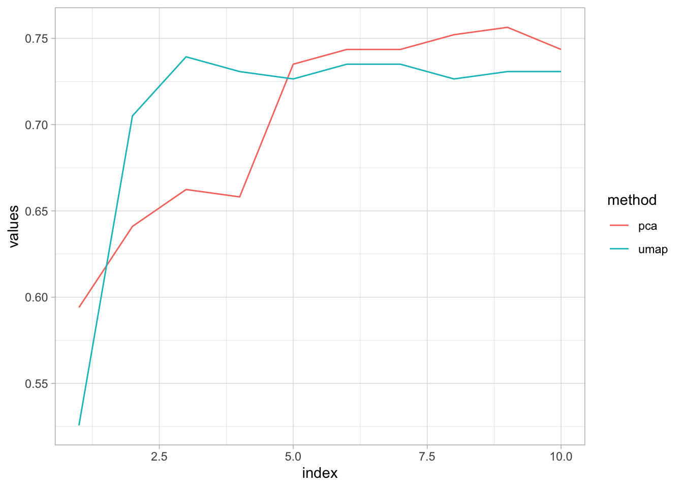

Seems like the accuracy converge at 75% as the number of components increase, actually after 5 components, PCA performs better than UMAP. Basically, PCA needs at least 5 components to get the height of UMAP.

library(microbenchmark)
time_UMAP <- microbenchmark(svm_test(3,"UMAP"), times = 10, unit="s")
time_PCA <- microbenchmark(svm_test(5,"PCA"), times = 10, unit="s")
cat("UMAP: ", mean(time_UMAP$time)/1e9, ", PCA: ", mean(time_PCA$time/1e9))

## UMAP:  2.005904 , PCA:  0.330938

Here is the result, PCA undoubtedly crushes UMAP. I know, I know, you mean that this is because the dataset is so small that the advantages of low dimensionality are not fully realezed, and this is just one example and doesn’t tell us much. I totally agree, I really am. What I would like to say is, the job of a data analyst should not be to blindly pursue new technologies, but to be flexible and efficient in getting tasks done.

Some of the code for the data mining section is taken from here, I’m very grateful to Julia Silge and David Robinson for their videos.

Leave a message if you like this blog.